Hello. Did you have any problems with optics or light?
Hikari learning aims to be a light source that transmits various information under the theme of “optics”. The sources of information are public information on the Internet and some knowledge and experience of the author. This page explains the questions that you always have when you start using OpticStudio, “What is ZDA files?” and “Points to be aware of with the analysis function”.
Conclusion
- The ZDA file stores the position and size of the editor and analysis windows that was open when saving the file, and the data of the analysis results. The ZDA file is always generated as a pair of .ZMX and .ZOS files with same file name.
- When using the analysis features, be sure to check the analysis condition settings before coonsidering the results.
Explanations of Session file, ZDA file
We often confirm layout window and analysis window during designing optical system and checking the optical performance. Knowing how to handle analysis data and how to use the analysis window in common will help operation of OpticStudio more efficiently.
***.ZDA (Session File)
OpticStudio uses many types of file extensions. The most important file is .ZMX or .ZOS file that contains editor data such as optical design and merit functions. And .ZDA file and .CFG file (user-created) that are automatically generated in the same folder.
The following knowledge bases are the answer to this question.
・ What are the .ZDA and .CFG Files?
・ Zemax file extensions
As a brief summary, the ZDA file contains the position and size of the editor and analysis window that was open when the file was saved, as well as the analysis result data. In other words, it does not contain any information about the optical design itself, and the role of the ZDA file is to “start up with the OpticStudio screen that you saw last time.” In other words, if you just want to share your optical design data, you can send only the .ZMX file and other OpticStudio users will be able to open the file. However, if there is no ZDA file, the only window that opens automatically is the Lens Data Editor.
Comments on sequential mode analysis functions
I explain some features introduced in the knowledge base articles. I’d like to add comments that can be applied common functions and analysis windows and the attitudes when using the analysis function.
First, let’s open “Settings”
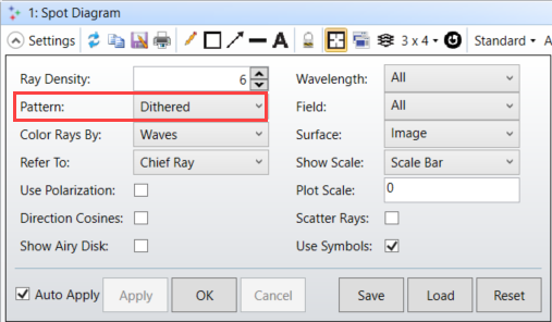
At the top left of almost all analysis windows, there is a “Settings” button that you can click to set the conditions for calculation the results displayed on the analysis screen. When you open the analysis window, it is highly recommended that you always check the conditions at the settings before you start considering the output results.
For example in the spot diagram, what is the parameter of the number of rays? Does the result change by increasing the number of rays? Is the wavelength setting appropriate? Are there any unclear setting parameters? Etc. I believe that touching every things will help you to understand the tools.
Simulation software, not only OpticStudio, is not a tool that tells you the correct result, but a tool that displays the calculation result under the conditions we set. We should determine if the calculation result is correct. The certainty of the calculation result depends on whether we set reasonable conditions for “setting”.
However, I know it’s hard to understand all the algorithms. The details of the computations done inside OpticStudio are a black box for us, and the software always has risk of bugs, and we need to consider the uncertainty. With the help of Zemax, forums and references from past heros, I hope to deepen our understanding of optics.
“Active cursor” is convenient, but assume it as a guide
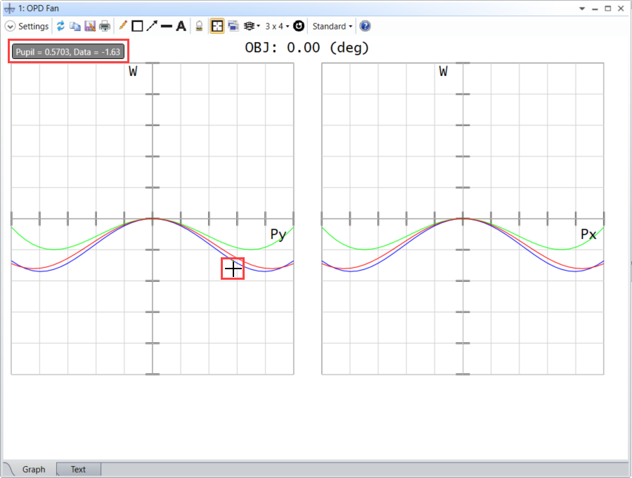
In the analysis window, there is a function called “active cursor” that displays the coordinate values in real time when you place the cursor on the graph. This function is very convenient because you can easily check the result without checking the result in text format.
However, I do not recommend overconfidence in that number. Depending on the resolution and zoomed state of the window, the values from active cursor may be inaccurate, even if we place the cursor over the plot exactly. Therefore, let’s just know the rough numerical value from active coursor and use the raw data of the analysis result stored in the text tab for detailed analysis.
Let’s compare the results from multiple algorithms
Some sequential mode analysis functions have several options that use multiple algorithms to output similar results. A typical example is MTF. There are three types of algorithms: geometrical MTF, FFT (Fast Fourier Transform) MTF, and Huygens MTF. Fiber couplings efficiency is from both of single-mode fiber coupling and physical optical propogation.
We always wonder which analysis function to be used. Unfortunately, there is no clear answer to this question such as “settings” discussion. OpticStudio doesn’t tell you which features is appropriate and which features will provide the most realistic results. We need to understand the prerequisites and constraints for each algorithm and choose the right features depending on the final application.
When we have concerning in output results, it’s a good idea to first output the results from another algorithm and compare them. If you confirm any clear difference, an algorithm with less approximation (less assumptions and constraints) is more likely to be the result. For example, if the optical system is close to the diffraction limit, the FFT result is less assumption than the geometrical optics, and the Huygens result is less assumption than the FFT. Conversely, if no difference is seen, it is advantageous to use an algorithm with a strong approximation. This is because geometrical optics has the fastest calculation speed and is highly robust to calculation conditions.
Simple illumination analysis is possible even in sequential mode
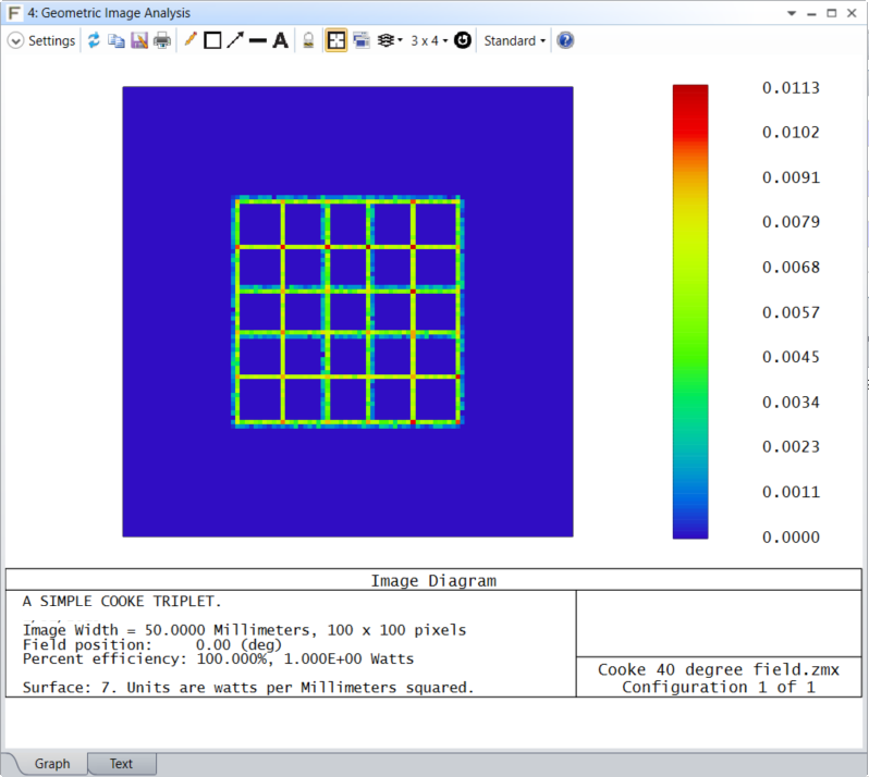
In Hikari learning, I explained that sequential mode is mainly for imaging optical system and non-sequential mode is used for illumination systems. However, OpticStudio’s sequential mode has the ability to enable simple illumination analysis. This is the “Extended Light Source Analysis” featured in the Knowledge Base article.
Sequential mode typically handle with rays from point sources, but these features allow you to set up a light source with a finite emission area. Compared to the non-sequential mode, the sequential mode enables high-speed ray tracing, and the ability to evaluate the imaging system and the illumination system in the same file has a great advantage in terms of work efficiency. However, since there are few options for the angular distribution of rays and there are strong restrictions on the handling of scattering, a non-sequential mode is required for detailed analysis.
“Illumination analysis is possible even in sequential mode.” Just knowing this may make your future OpticStudio life more comfortable.
Summary
Here, I explained on outline of the ZDA file related to the analysis function of OpticStudio and the attitude to use the analysis function were explained. The latter half includes a lot of my personal subjectivity, so please consider it as one opinion on OpticStudio.


コメント